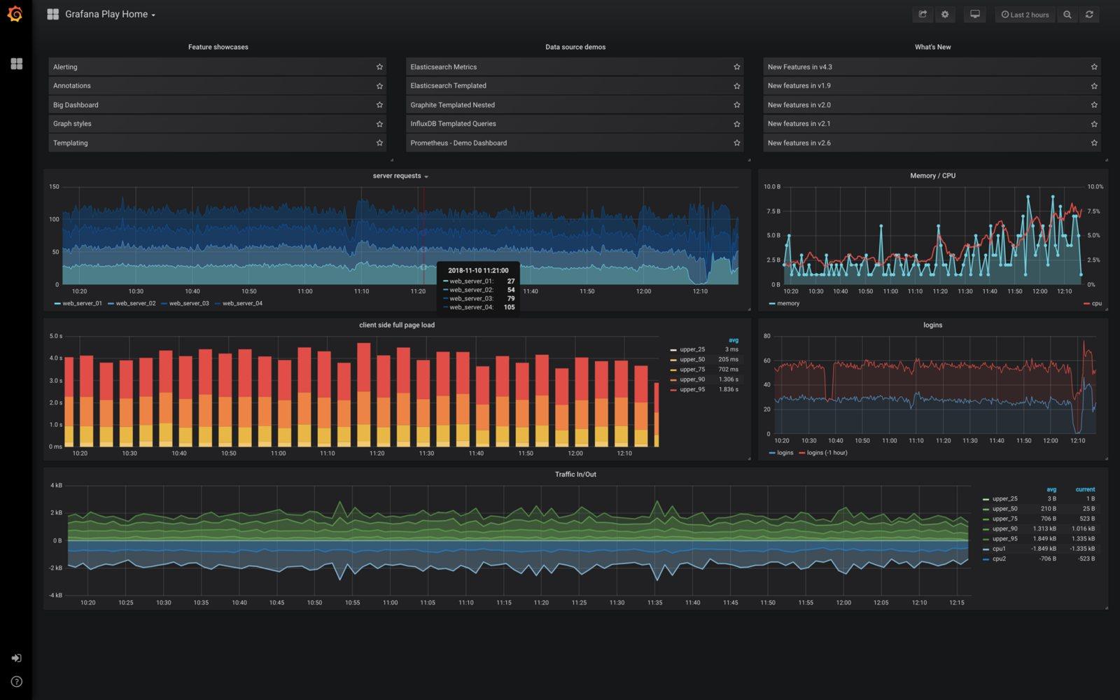
Walk into any shop that pays for machine monitoring and you'll see the same thing on the wall: a row of machines, each with a coloured timeline: green for running, yellow for idle, red for alarm. It's genuinely useful. It's also, under the hood, a database of state changes and a charting tool. Both are free.
This post builds that wall screen with Grafana (open source, AGPLv3) and PostgreSQL, fed by a small Python collector. It assumes your machines already speak MTConnect, natively or through an adapter like the one in setting up an MTConnect agent for a legacy CNC. Everything here runs on one modest PC or VM.
MTConnect agents --> collector.py (poll /current every 2 s, store CHANGES only)
                         |
                    PostgreSQL  (machine_state, machine_sample)
                         |
                      Grafana   (state timeline, utilization, alerts, TV kiosk)
Why PostgreSQL and not a time-series database?
InfluxDB and friends are excellent at high-rate sensor data, and if you're sampling vibration at kilohertz rates, use one. But machine state is low-rate and relational: a machine changes state maybe a few hundred times a shift, and the questions you'll ask ("utilization by machine by shift, excluding planned maintenance, joined to the job schedule") are SQL questions. Plain PostgreSQL handles years of state history for a 30-machine shop without breaking a sweat, and you already know how to back it up. If the sample tables grow huge later, the TimescaleDB extension drops in without changing your queries.
Step 1: run the stack
# docker-compose.yml
services:
  db:
    image: postgres:17
    environment:
      POSTGRES_DB: shopfloor
      POSTGRES_USER: shop
      POSTGRES_PASSWORD: change-me
    volumes: [pgdata:/var/lib/postgresql/data]
    ports: ["5432:5432"]
  grafana:
    image: grafana/grafana-oss
    ports: ["3000:3000"]
    volumes: [grafana:/var/lib/grafana]
    depends_on: [db]
volumes: { pgdata: {}, grafana: {} }
docker compose up -d, then open http://<host>:3000, log in, and add a PostgreSQL data source pointing at db:5432. Pin the Grafana image to a specific version once it's working: dashboards are stable across releases, but you don't want a surprise major upgrade the morning of a customer audit.
Step 2: two tables, designed for the questions
-- one row per state CHANGE, not per poll
CREATE TABLE machine_state (
  machine    text        NOT NULL,
  ts         timestamptz NOT NULL,
  execution  text        NOT NULL,   -- ACTIVE, READY, INTERRUPTED, STOPPED, UNAVAILABLE...
  mode       text,
  program    text,
  part_count integer,
  PRIMARY KEY (machine, ts)
);

-- numeric samples (spindle load, feed override...) at whatever rate you poll
CREATE TABLE machine_sample (
  machine text        NOT NULL,
  ts      timestamptz NOT NULL,
  name    text        NOT NULL,
  value   double precision,
  PRIMARY KEY (machine, name, ts)
);
Storing changes only is the decision that keeps this fast. A machine polled every two seconds generates 43,200 rows a day if you store every poll; storing changes, it's a few hundred. Each row implicitly lasts until the next row for that machine, and a SQL window function recovers durations whenever you need them.
Step 3: the collector
# collector.py - pip install requests psycopg[binary]
import time, xml.etree.ElementTree as ET
from datetime import datetime, timezone
import psycopg, requests

AGENTS = {"DMU50-Cell3": "http://192.168.20.10:5000/DMU50-Cell3/current",
          "Mazak-2":     "http://192.168.20.11:5000/current"}

def read(url):
    root = ET.fromstring(requests.get(url, timeout=3).content)
    val = lambda tag: (root.find(f".//{{*}}{tag}") is not None
                       and root.find(f".//{{*}}{tag}").text) or None
    return {"execution": val("Execution") or "UNAVAILABLE",
            "mode": val("ControllerMode"), "program": val("Program"),
            "part_count": int(val("PartCount")) if (val("PartCount") or "").isdigit() else None}

last = {}
with psycopg.connect("postgresql://shop:change-me@localhost/shopfloor", autocommit=True) as db:
    while True:
        now = datetime.now(timezone.utc)
        for machine, url in AGENTS.items():
            try:
                s = read(url)
            except (requests.RequestException, ET.ParseError):
                s = {"execution": "UNAVAILABLE", "mode": None, "program": None, "part_count": None}
            if s != last.get(machine):          # store changes only
                db.execute("INSERT INTO machine_state VALUES (%s,%s,%s,%s,%s,%s)",
                           (machine, now, s["execution"], s["mode"], s["program"], s["part_count"]))
                last[machine] = s
        time.sleep(2)
The {*} namespace wildcard is what lets one parser read agents running different MTConnect schema versions. And note the failure path: if an agent is unreachable, the collector records UNAVAILABLE rather than silently keeping the last known state. A dashboard that shows a dead connection as "running" is worse than no dashboard.
Step 4: the panels that matter
Resist the urge to build forty panels. A shop-floor screen read from ten metres away needs four things:
- 1State timeline: one coloured bar per machine across the shift. This is the panel everyone looks at.
- 2Utilization % (Stat): share of the selected window each machine spent
ACTIVE, big numbers, colour-thresholded. - 3Parts this shift (Bar gauge): from
part_countdeltas. - 4Currently stopped (Table): which machines are down right now, and for how long, sorted longest first.
For the state timeline, query the raw change rows and let Grafana draw them. Add a Partition by values transformation on the machine column to get one row per machine, then use value mappings to colour ACTIVE green, READY/INTERRUPTED amber, STOPPED red, and UNAVAILABLE grey:
SELECT ts AS time, machine, execution
FROM machine_state
WHERE ts BETWEEN $__timeFrom()::timestamptz - interval '1 day' AND $__timeTo()::timestamptz
ORDER BY ts
(The extra day pulls in the state each machine was already in when the window opened, so the first bar isn't blank.) Utilization is where the window function earns its keep: compute each state's duration, clip it to the dashboard's time range, and sum the active time:
WITH spans AS (
  SELECT machine, execution,
         GREATEST(ts, $__timeFrom()::timestamptz) AS t0,
         LEAST(LEAD(ts, 1, now()) OVER (PARTITION BY machine ORDER BY ts),
               $__timeTo()::timestamptz)           AS t1
  FROM machine_state
)
SELECT machine,
       100 * SUM(EXTRACT(EPOCH FROM t1 - t0)) FILTER (WHERE execution = 'ACTIVE')
           / NULLIF(SUM(EXTRACT(EPOCH FROM t1 - t0)), 0) AS utilization
FROM spans
WHERE t1 > t0
GROUP BY machine
ORDER BY machine
Utilization is not OEE
This number is time running ÷ time observed, which is the honest version of what most wall screens show. OEE also needs planned time, ideal cycle time, and good-part counts. OEE from scratch walks through the formula, and the OEE calculator lets you sanity-check the numbers this query feeds it.
Step 5: alerts and the wall screen
- Alert on duration, not on events. "Machine STOPPED for more than 15 minutes during a shift" is actionable; "machine changed state" is spam. Grafana alert rules can evaluate the "currently stopped" query every minute and notify by email, Teams, or Slack.
- Kiosk mode. Append
?kioskto the dashboard URL on the TV's browser to hide all chrome, and set the time range to "Today so far" with a 30 s refresh. - Read-only access. Give the TV a Viewer account. The wall screen should never be one misclick away from deleting a panel.
- Annotations for context. Write planned maintenance and changeovers to a small
eventstable and show them as annotations, so a red bar during a scheduled PM doesn't start an argument.
What I'd add next
Once state history exists, the interesting questions arrive on their own. Join machine_state to your job schedule and you get utilization by part number. Collect machine_sample spindle load and you can trend it per tool, the raw material for predicting tool wear. Add a $50 accelerometer and vibration trends land on the same screen. Every one of those is a SQL query away, because the foundation is a database you own.
The value of a machine dashboard isn't the screen. It's the database underneath that, for the first time, remembers what every machine did.